Abstract
Batteries are electrochemical energy storage devices that exhibit physico-chemical heterogeneity on a continuity of scales. As such, battery systems are amenable to mathematical descriptions on a multiplicity of scales that range from atomic to continuum. In this paper we present a new method to assess the veracity of macroscopic models of lithium-ion batteries. Macroscopic models treat the electrode as a continuum and are often employed to describe the mass and charge transfer of lithium since they are computational tractable and practical to model the system at the cell scale. Yet, they rely on a number of simplifications and assumptions that may be violated under given operating conditions. We use multiple-scale expansions to upscale the pore-scale Poisson-Nerst-Planck (PNP) equations and establish sufficient conditions under which macroscopic dual-continua mass and charge transport equations accurately represent pore-scale dynamics. We propose a new method to quantify the relative importance of three key pore-scale transport mechanisms (electromigration, diffusion and heterogenous reaction) by means of the electric Péclet (Pe) and Damköhler (Da) numbers in the electrolyte and the electrode phases. For the first time, applicability conditions of macroscopic models through a phase diagram in the (Da-Pe)-space are defined. Finally, we discuss how the new proposed tool can be used to assess the validity of macroscopic models across different battery chemistry and conditions of operation. In particular, a case study analysis is presented using commercial lithium-ion batteries that investigates the validity of Newman-type macroscopic models under temperature and current rate of charge/discharge variation.
This is an open access article distributed under the terms of the Creative Commons Attribution 4.0 License (CC BY, http://creativecommons.org/licenses/by/4.0/), which permits unrestricted reuse of the work in any medium, provided the original work is properly cited.
Predictive understanding of battery dynamical behavior still remains a major bottleneck in achieving diagnostic capabilities, safety, optimization and control of battery systems under different operating conditions. Such a difficulty arises from two main factors: i) nonlinearity of lithium-ion transport processes1 and ii) battery systems multiscale structure that exhibits physicochemical heterogeneity on a continuity of scales (from the nanometer to the meter).2–5 Since the seminal work by Newman and Tiedemann,6 where macroscopic ion transport equations were first formulated, a plethora of models have spurred in the past decades. They range from fully empirical approaches to generalizations of electrochemical models based on the porous electrode theory to account for concentrated solutions,7,8 thermal effects9 and capacity fade due to Solid-Electrolyte Interphase (SEI)-growth,10–12 just to mention a few. In the past decade, ever increasing computational capabilities have fuelled the development of fully molecular/atomistic models and multiscale/multiphysics approaches.13 For a thorough review on the topic, we refer the reader to Ref. 4.
Microscale models14,15 (e.g. molecular dynamics, kinetic Monte Carlo and pore-scale models) are theoretically robust, but are impractical as a predictive tool at the system level due to their computational burden. For example, current molecular dynamics simulations are still prohibitive at the nano-second timescale.4,16 Such computational limitations become dire when modeling battery lifetime and slow degradation processes over hundreds or thousands of cycles. Further, the need for real-time estimation of battery State-of-Charge (SOC) and State-of-Health (SOH) currently limits the application of more accurate and computationally intensive models in favor of simpler macroscopic (effective, coarse-grained, continuum, etc.)17,18 and/or reduced-order representations.19,20
Macroscopic approaches overcome some of the computational challenges of microscale models by relying on a number of closure assumptions and/or phenomenological descriptions such as geometrical constraints that guarantee scale separation between the pore- and the continuum-scales, linearization of pore-scale equations, etc. These are often necessary to fully decouple micro-scale descriptions from their continuum counterpart. Yet, physical and electrochemical phenomena on one scale (e.g. particle-scale) affect, and are often coupled to, phenomena on a vastly different scale (e.g. cell-scale).21–23 For example, pore-scale molecular diffusion fundamentally affects lithium-ion mixing and heat generation at the electrode scale,9 and localized SEI-growth in the pores (over time scales spanning many orders of magnitude) can lead to drastic porosity changes and long term impairment (e.g. aging and capacity fade) of battery systems. Further, dependence of battery aging processes on usage patterns20,24 (i.e. charge and dischrage cycles amplitude and frequency) are often symptoms of coupled dynamics across scales.25
Upscaling techniques - e.g. volume-averaging,26 homogenization27 and its generalization to evolving microstructures,28 thermodynamically-constrained averaging29 and renormalization group theory30 - allow one to relate pore-scale processes to their continuum counterparts. An increasing number of studies have focused on the formal derivation of continuum-scale models from micro-scale balance equations.31–35 These studies reflect the need to validate reduced-order models and to elucidate the macroscopic response of microscale processes. Yet, to the best of our knowledge, no current work has rigorously established the conditions under which pore-scale equations describing electromigration, diffusion and reaction of lithium ions correctly upscale to the classical macroscopic porous-electrode equations. The identifications of conditions under which continuum approaches are a valid representation of microscopic processes is critical to achieve model predictivity of battery systems.
Following the approach introduced by,22,23 we use multiple-scale expansions technique to upscale the dimensionless PNP equations describing lithium dynamics and to derive physics-based conditions under which classical porous-electrode continuum models, or dual-continua diffusion-migration-reaction (DMR) equations, accurately describe lithium-ion pore-scale dynamics.
The paper is structured as follows. First, we present the pore-scale isothermal transport model of lithium ions subject to diffusion and electromigration in the electrode and electrolyte phases, and heterogenous Butler-Volmer kinetic reaction at the electrode-electrolyte interface. Then, we formulate the problem in dimensionless form and identify the Damköhler (Da) and electric Péclet (Pe) numbers as parameters that control lithium-ion transport processes (i.e. diffusion, electromigration and reaction) in the electrode and electrolyte. We employ multiple-scale expansions to derive effective (macroscopic) dual-continua DMR equations and rigorously identify conditions under which such a continuum approximation breaks down. The region of validity of the continuum description is graphically represented by two phase diagrams in the (Da, Pe) space for the electrode and the electrolyte phases. Then, we discuss the implications of our findings on the classical porous-electrode model proposed by Doyle and Newman.8 Lastly, we present a case study analysis to investigate the validity of macroscale models in relations to: 1) different chemistry, and 2) different conditions of operation in terms of temperature and C-rate for a series of commercially available batteries. We achieve this by relating macroscale models' predictive performance to the applicability regimes. Finally, we conclude with a summary of our results.
Pore-Scale Governing Equations
We consider the microscale transport of lithium ions in a battery electrode constituted of a porous matrix  with characteristic length L. Let us assume that the active particles are microscopically arranged in the medium in the form of spatially periodic unit cells
  with a characteristic length ℓ. We define the characteristic length ℓ as the diameter of the spherical active particles and ε as the scale-separation parameter ε ≡ ℓ/L ≪ 1. The unit cell
  consists of the electrolyte space
  and the ion permeable solid matrix
  , separated by the smooth surface
  . The pore spaces
  of each cell
  form a multi-connected pore-space domain
  bounded by the smooth surface
  .
.
The mass and charge transport equations in the electrolyte and the electrode phases control the spatiotemporal evolution of the concentration of lithium ions  (mol · m− 3) and the electrostatic potential
  (V) in the active particles {i = s} and the electrolyte {i = e}. For completeness, we summarize the set of governing equations in the following sections.
Electrolyte phase
The mass and charge transport equations in the electrolyte phase  are36
are36
![Equation ([1a])](https://content.cld.iop.org/journals/1945-7111/162/10/A1940/revision1/jes_162_10_A1940eqn1.jpg)
![Equation ([1b])](https://content.cld.iop.org/journals/1945-7111/162/10/A1940/revision1/jes_162_10_A1940eqn2.jpg)
subject to
![Equation ([2a])](https://content.cld.iop.org/journals/1945-7111/162/10/A1940/revision1/jes_162_10_A1940eqn3.jpg)
![Equation ([2b])](https://content.cld.iop.org/journals/1945-7111/162/10/A1940/revision1/jes_162_10_A1940eqn4.jpg)
on the solid-electrolyte boundary Γε, respectively. In (2),
![Equation ([3])](https://content.cld.iop.org/journals/1945-7111/162/10/A1940/revision1/jes_162_10_A1940eqn5.jpg)
 (m2sec− 1) and
  (Ω− 1m− 1) are the interdiffusion coefficient and the electric conductivity in the electrolyte, respectively; k (A · m · mol− 1) is the electrochemical reaction rate constant that describes the kinetics of lithium-ion transfer on Γε;
  (V) is the open circuit potential;
  is the maximum concentration of lithium that can be stored in the active particle; t+ is the transference number,
  is assumed constant,37 and f± is the activity coefficient; ne is the outward unit normal vector to
  pointing from the electrolyte toward the active particle; F and R are the Faraday and the universal gas constants; T is temperature.
Electrode phase
The mass and charge transport of lithium ions in the electrode (solid) phase  are governed by the material balance and electroneutrality equations36
![Equation ([4a])](https://content.cld.iop.org/journals/1945-7111/162/10/A1940/revision1/jes_162_10_A1940eqn6.jpg)
![Equation ([4b])](https://content.cld.iop.org/journals/1945-7111/162/10/A1940/revision1/jes_162_10_A1940eqn7.jpg)
subject to
![Equation ([5a])](https://content.cld.iop.org/journals/1945-7111/162/10/A1940/revision1/jes_162_10_A1940eqn8.jpg)
![Equation ([5b])](https://content.cld.iop.org/journals/1945-7111/162/10/A1940/revision1/jes_162_10_A1940eqn9.jpg)
respectively. In (4)-(5),  (m2sec− 1) is the interdiffusion coefficient in the electrode,
  (Ω− 1m− 1) is the electric conductivity in the electrode, and ns is the outward unit normal vector to Γε pointing from the active particle toward the electrolyte.
Dimensionless Formulation
Transport processes and dimensionless numbers
The transport processes occurring at the pore-scale include heterogenous reaction on the electrode-electrolyte interface  , and diffusion and migration in the electrode and electrolyte phases,
  and
and  , respectively. The characteristic time scales associated with the heterogenous reaction, ionic diffusion, and ionic migration over a macroscopic length scale L are
![Equation ([6])](https://content.cld.iop.org/journals/1945-7111/162/10/A1940/revision1/jes_162_10_A1940eqn10.jpg)
respectively. In (6),  and
and  , j = {e, s}, are characteristic values of the interdiffusion and electric conductivity tensors
  and
and  in the electrode (j = s) and the electrolyte (j = e), respectively. We define the dimensionless Damköhler and electric Péclet numbers as
![Equation ([7])](https://content.cld.iop.org/journals/1945-7111/162/10/A1940/revision1/jes_162_10_A1940eqn11.jpg)
They provide information about the relative magnitude of ion transport processes in the electrolyte and the electrode phases. Let  and
and  , j = {s, e} be the dimensionless lithium-ion concentration and electrostatic potential in the active particles (j = s) and the electrolyte (j = e). Then, the mass and charge transport equations can be cast in dimensionless form as follows.
Electrolyte phase
The dimensionless form of mass and charge transport in the electrolyte (1)-(2) is given by
![Equation ([8a])](https://content.cld.iop.org/journals/1945-7111/162/10/A1940/revision1/jes_162_10_A1940eqn12.jpg)
![Equation ([8b])](https://content.cld.iop.org/journals/1945-7111/162/10/A1940/revision1/jes_162_10_A1940eqn13.jpg)
subject to
![Equation ([9a])](https://content.cld.iop.org/journals/1945-7111/162/10/A1940/revision1/jes_162_10_A1940eqn14.jpg)
![Equation ([9b])](https://content.cld.iop.org/journals/1945-7111/162/10/A1940/revision1/jes_162_10_A1940eqn15.jpg)
on Γε, respectively. In (1) and (2), the dimensional spatial and time scales are nondimensionalized by the macroscopic length L and the diffusion time in the electrolyte phase  respectively, i.e.
  and
and  ;
;  and
and  are the dimensionless interdiffusion coefficient and the electric conductivity in the electrolyte. Also,
![Equation ([10])](https://content.cld.iop.org/journals/1945-7111/162/10/A1940/revision1/jes_162_10_A1940eqn16.jpg)
where  is the dimensionless open circuit potential. We emphasize that
  and
and  represent the rescaled (nondimensional) electrolyte and electrode phases, with Γε the interface separating them.
Electrode phase
Similarly, the dimensional transport equations in the electrode phase  , (4) and (5), can be cast in dimensionless form
![Equation ([11a])](https://content.cld.iop.org/journals/1945-7111/162/10/A1940/revision1/jes_162_10_A1940eqn17.jpg)
![Equation ([11b])](https://content.cld.iop.org/journals/1945-7111/162/10/A1940/revision1/jes_162_10_A1940eqn18.jpg)
subject to
![Equation ([12a])](https://content.cld.iop.org/journals/1945-7111/162/10/A1940/revision1/jes_162_10_A1940eqn19.jpg)
![Equation ([12b])](https://content.cld.iop.org/journals/1945-7111/162/10/A1940/revision1/jes_162_10_A1940eqn20.jpg)
respectively.
In the following we use multiple-scale expansions to derive a mean-field (continuum, macroscopic) approximation of the pore-scale equations and to identify conditions under which continuum equations are valid descriptors of pore-scale dynamics.
Homogenization via Multiple-Scale Expansions
We define the following local averages of a quantity 
![Equation ([13])](https://content.cld.iop.org/journals/1945-7111/162/10/A1940/revision1/jes_162_10_A1940eqn21.jpg)
![Equation ([14])](https://content.cld.iop.org/journals/1945-7111/162/10/A1940/revision1/jes_162_10_A1940eqn22.jpg)
![Equation ([15])](https://content.cld.iop.org/journals/1945-7111/162/10/A1940/revision1/jes_162_10_A1940eqn23.jpg)
where  ,
,  and
and  is the electrode porosity. Using the method of multiple-scale expansions, we introduce a fast space variable y defined in the unit cell Y, y ∈ Y, and three time variables. One of the three time variables is related to reaction τr and two to migration
  in the electrolyte and the active particles j = {e, s}, respectively
![Equation ([16])](https://content.cld.iop.org/journals/1945-7111/162/10/A1940/revision1/jes_162_10_A1940eqn24.jpg)
where  is a dimensionless time. No Einstein notation convention is implied if a repeated index is present. Replacing any pore scale quantity ψε(x, t) (e.g. concentration, electrostatic potential in either phase) with
  provides the following relations for the space and time derivatives,
![Equation ([17a])](https://content.cld.iop.org/journals/1945-7111/162/10/A1940/revision1/jes_162_10_A1940eqn25.jpg)
![Equation ([17b])](https://content.cld.iop.org/journals/1945-7111/162/10/A1940/revision1/jes_162_10_A1940eqn26.jpg)
Additionally, we represent ψ as an asymptotic series in integer powers of ε
![Equation ([18])](https://content.cld.iop.org/journals/1945-7111/162/10/A1940/revision1/jes_162_10_A1940eqn27.jpg)
where ψn, n = {0, 1, ⋅⋅⋅} are Y-periodic functions in y. Finally, we set
![Equation ([19])](https://content.cld.iop.org/journals/1945-7111/162/10/A1940/revision1/jes_162_10_A1940eqn28.jpg)
where the exponents α, β, γ and δ determine the system behavior in the electrolyte and electrode phases.
Upscaled transport equations in the electrolyte
Lithium transport in the electrolyte phase described by (8a)–(9b) can be homogenized, i.e., approximated up to order ε2, by the following effective mass and charge transport equations (see Appendix A)
![Equation ([20])](https://content.cld.iop.org/journals/1945-7111/162/10/A1940/revision1/jes_162_10_A1940eqn29.jpg)
and
![Equation ([21])](https://content.cld.iop.org/journals/1945-7111/162/10/A1940/revision1/jes_162_10_A1940eqn30.jpg)
where
![Equation ([22])](https://content.cld.iop.org/journals/1945-7111/162/10/A1940/revision1/jes_162_10_A1940eqn31.jpg)
provided the following conditions are met:
- (1)ε ≪ 1,
- (2)Dae < 1,
- (3)Pee < 1,
- (4)Dae/Pee < 1,
- (5)
 .
.
In (20) and (21), the dimensionless effective reaction rate constant in the electrolyte phase,  , is determined by the pore geometry,
![Equation ([23])](https://content.cld.iop.org/journals/1945-7111/162/10/A1940/revision1/jes_162_10_A1940eqn32.jpg)
and the dispersion tensors are given by:
![Equation ([24])](https://content.cld.iop.org/journals/1945-7111/162/10/A1940/revision1/jes_162_10_A1940eqn33.jpg)
The closure variable  has zero mean,
  , and is defined as a solution to the local problem
![Equation ([25a])](https://content.cld.iop.org/journals/1945-7111/162/10/A1940/revision1/jes_162_10_A1940eqn34.jpg)
![Equation ([25b])](https://content.cld.iop.org/journals/1945-7111/162/10/A1940/revision1/jes_162_10_A1940eqn35.jpg)
Constraints 1)–4) ensure separation of scales. While constraint 1) is almost always met in practical applications since the pore size is generally much smaller that the electrode dimension, constraints 2)–4) depend on the relative importance of the diffusion, electromigration, and reaction mechanisms, i.e. they impose constraints on the transport regimes that can be appropriately modeled by the continuum scale Equations (20) and (21) within errors of order ε2. These conditions are summarized in the phase diagram in Figure 1, where the line β = 0 refers to Dae = 1 and the half-space β > 0 refers to Dae < 1 because ε < 1; the line α = 0 refers to Pee = 1 and the half-space αe < 0 refers to Pee < 1; the line α + β = 0 refers to Dae/Pee = 1; and the half-space underneath this line refers to Dae/Pee < 1. Constraint 5) is not necessary for scale separation, but facilitates the derivation of the effective parameters (23) and (24). As shown in Appendix A, this constraint allows one to interchange the surface and volume averages,  and
and 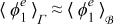 , within errors on the order of ε2.
Figure 1. Phase diagram specifying the range of applicability of the upscaled Equations (20) and (21) for the diffusion-migration-reaction of lithium ions in the electrolyte in terms of Pee and Dae. The gray region identifies the conditions under which the macro-scale Equations (20) and (21) hold. In the white region, micro- and macro-scale equations are coupled and need to be solved simultaneously. Diffusion, migration, and reaction are of the same order of magnitude at the point (α, β) = (0, 0).
Upscaled transport equations in the electrode
In Appendix B, we show that the microscale reactive transport processes described by (11)–(12) can be homogenized, i.e., approximated up to order ε2 in the solid phase with an effective mass and charge transport equations
![Equation ([26])](https://content.cld.iop.org/journals/1945-7111/162/10/A1940/revision1/jes_162_10_A1940eqn36.jpg)
and
![Equation ([27])](https://content.cld.iop.org/journals/1945-7111/162/10/A1940/revision1/jes_162_10_A1940eqn37.jpg)
for x ∈ Ω, provided the additional conditions
- (1)Das < 1,
- (2)Das/Pes < 1,
- (3),
are met. In (26) and (27), the dimensionless parameter  is defined by (23) and the effective diffusion and conductivity tensors are given by
![Equation ([28])](https://content.cld.iop.org/journals/1945-7111/162/10/A1940/revision1/jes_162_10_A1940eqn38.jpg)
The closure variable  has zero mean,
  , and is defined as a solution of the local problem
![Equation ([29a])](https://content.cld.iop.org/journals/1945-7111/162/10/A1940/revision1/jes_162_10_A1940eqn39.jpg)
![Equation ([29b])](https://content.cld.iop.org/journals/1945-7111/162/10/A1940/revision1/jes_162_10_A1940eqn40.jpg)
Constraints 1)–2) ensure scales separation and depend on the relative importance of the solid phase diffusion, conduction, and reaction mechanisms of transport. Condition 3) simply facilitates the derivation of the effective tensor (28). These constraints are summarized in Figure 2.
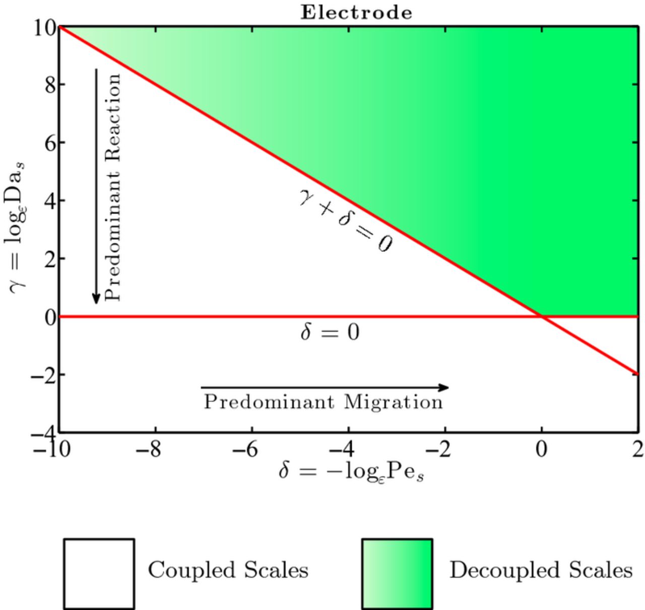
Figure 2. Phase diagram specifying the range of applicability of the upscaled Equations (26) and (27) for the diffusion-reaction of lithium ions in the electrode in terms of Pes and Das. The gray region identifies the conditions under which the macro-scale Equations (26) and (27) hold. In the white region, micro- and macro-scale equations are coupled and need to be solved simultaneously. Diffusion and reaction are of the same order of magnitude at the point (δ, γ) = (0, 0).
Physical interpretation of applicability conditions of macroscopic models
The constraints previously identified impose conditions on the relative magnitude of the three main processes controlling lithium-ion transport at the microscale, i.e. diffusion, electromigration and heterogenous reaction at the electrolyte-electrode interface. The constraints Dae < 1 and Das < 1 require that the intercalation reaction be slower than diffusion processes both in the electrolyte and the electrode. Similarly Pee < 1 requires that diffusion processes in the electrolyte are faster than elecromigration. Both conditions guarantee that lithium ions are uniformly distributed, i.e. well mixed, both in the pore-space occupied by the electrolyte and within electrode pellets at the unit cell scale. Under well-mixed conditions, or when lithium-ion concentration is locally uniform, a dual-continua macroscale model can describe processes at the micro-scale within errors of order  as prescribed by the homogenization procedure. On the other hand, under diffusion-limited conditions, or high resistance to mass transport, concentration gradients are formed at the sub-pore scale, and the predictivity of continuum scale models, which replace pore-scale quantities with their spatial averages, cannot be guaranteed any longer. Our findings are consistent with the widespread observation that classical macroscopic approximations loose predictive power under high C-ratec operating conditions,39 when a strong current imbalance between electrodes generates sharp concentration gradients at the sub pore level. The importance of lack of subpore scale mixing was already pointed out in Ref. 9, where subgrid concentration gradients were associated with generation of highly localized heat of mixing. The constraints Dae/Pee < 1 and Das/Pes < 1 suggest that elecromigration can play a favorable role in improving the sub-pore scale mixing in presence of high mass transfer resistance, or diffusion-limited regimes. Finally, the dependence of Pee and Pes on the operating temperature, see (7), demonstrates that isothermal conditions are not sufficient to guarantee macroscale model accuracy: operating the same battery at a higher temperature may lead to the violation of Pee < 1 and/or Pes < 1, once a critical temperature is overcome. A more thorough analysis of temperature-dependent breakdown for different battery chemistry is discussed in the next section as well as in Ref. 40. In the following section, we discuss the implications of our findings on existing dual continua models.
Implications on Existing Macroscale Models for SOC and SOH Estimation
A number of works have focused on control strategies and SOH/SOC estimation based on electrochemical models.39,41,42 Some of the most popular models on which Partial Differential Equation (PDE) control and estimation strategies are based upon are, e.g., Newman's model,8 its generalizations43 and the single particle model (SPM).44 Such models have the advantage of being relatively simple for controller/observer design as they are classical macroscopic/upscaled models which treat the complex porous structure and the electrolyte as superimposed fully-connected continua.
For example, the SPM is based on the key idea that the solid phase of each electrode can be idealized as a single spherical particle, while the electrolyte lithium-ion concentration is constant in space and time.44 Its governing equations therefore reduce to Fick's law in spherical coordinates and can be readily derived from (20)-(21) and (26)-(27) under the appropriate model assumptions (e.g. constant  and negligible electromigration). Similarly, Newman's model8 can be obtained from (20)-(21) and (26)-(27) by relaxing the assumption that
  is approximately constant and including the full mass transport equation in the electrolyte phase (20), while still assuming negligible electromigration.
As such, these models are based on the fundamental, and often untested, assumption that separation of scales occurs and, consequently, macroscopic representations of averaged quantities can describe pore-scale processes with an accuracy prescribed by mathematical homogenization. Yet, since their validity is limited to the same constraints identified in Figures 1 and 2, they should be used with caution when the sufficient conditions listed above are violated. In the following section, we demonstrate the use of the phase diagrams in Figures 1 and 2 to a priori estimate macroscale models accuracy compared to their fully resolved counterparts for commercial battery systems.
Case Study for Commercial Batteries: Validity of Macroscale Models
In this section, we investigate the validity of macroscale models in relations to: 1) different chemistry, and 2) different conditions of operation in terms of temperature and C-rate for a series of commercially available batteries. In particular, we compare the accuracy of continuum-scale models with either their fully resolved (3D) counterparts or with experiments as reported in a number of studies.45–51 More importantly, we relate macroscale models' predictive performance to the applicability regimes defined in Figures (1) and (2), and employ the former as a screening tool to a priori evaluate continuum model predictivity under variable C-rate.
Chemistry dependence of macroscale models
The battery cell parameter data used in this case study, and reported in Table I, are based on a variety of electrode and electrolyte compositions at room temperature (T = 298 K).45–51 The dimensionless parameters α, β, γ and δ in the electrolyte and electrode phases, readily calculated from (7) and (19), are reported in Table II and plotted on the corresponding phase diagram for the electrolyte and electrode, Figure 3 and 4, respectively.
Table I. Lithium-ion battery parameters for both electrode and electrolyte phases as reported in Refs. 45–51. Values of k reported in Refs. 45–51 have been appropriately normalized by F and cmax such that the dimensions of k are consistent with (2).
| Electrode | ℓ [m] | L [m] | ε [-] | k [A · m · mol− 1] | cmax [mol · m− 3] | De [m2sec− 1] | Ke [Ω− 1m− 1] | Ds [m2sec− 1] | Ks [Ω− 1m− 1] | Ref. |
|---|---|---|---|---|---|---|---|---|---|---|
| LiC6 | 1.02e-6 | 9.85e-5 | 1.04e-2 | 6.15e-4 | 26000 | 3.94e-11 | 0.192 | 9.89e-14 | 100 | 45 |
| LiC6 | 2.5e-5 | 1.62e-4 | 0.154 | 7.5e-4 | 28200 | 2.93e-10 | 1.29 | 1e-13 | 100 | 46 |
| LiC6 | 2e-6 | 7.9e-5 | 0.025 | 3.02e-4 | 31540 | 2.3e-10 | 1.323 | 3.9e-14 | 2 | 47 |
| LixC6 | 2e-5 | 1.13e-4 | 0.177 | 3.11e-4 | 26000 | 2.6e-10 | 1 | 3.9e-14 | 100 | 48 |
| Li1 − xC6 | 2e-6 | 3.7e-5 | 0.054 | 1.75e-2 | 16,100 | 2.6e-10 | 5.676 | 2e-16 | 100 | 49 |
| LiCoO2 | 2e-5 | 1.05e-4 | 0.190 | 4.36e-4 | 51000 | 2.6e-10 | 1 | 1e-13 | 100 | 48 |
| LiFePO4 | 3.31e-8 | 9.5e-5 | 3.48e-4 | 1.15e-4 | 22806 | 3.94e-11 | 0.192 | 4.29e-18 | 0.49 | 45 |
| LiFePO4 | 2e-6 | 1.12e-4 | 0.152 | 5.68e-4 | 26390 | 2.3e-10 | 1.323 | 1.25e-15 | 0.01 | 47 |
| Li4Ti5O12 | 1.075e-8 | 9.6e-5 | 1.12e-4 | 1.49e7 | 51385 | 2e-10 | 0.38 | 6.8e-15 | 100 | 50,51 |
| LiNi1/3Mn1/3Co1/3O2 | 2.4e-6 | 8.6e-5 | 0.028 | 9.92e-3 | 51385 | 2e-10 | 0.38 | 2.5e-16 | 139 | 50,51 |
| LiNi0.8Co0.2 − xAlxO2 | 8e-6 | 8.6e-5 | 0.093 | 5.5e-3 | 49195 | 2.93e-10 | 1.29 | 2e-13 | 10 | 46 |
| LixNiyCozAl1 − y − zO2 | 2.5e-6 | 2.9e-5 | 0.086 | 9.76e-3 | 23,900 | 2.6e-1 | 5.676 | 3.7e-16 | 10 | 49 |
Table II. Dimensionless transport parameters calculated from (7) and (19) for the battery chemistry listed in Table I.
| Electrode | Dae [-] | Pee [-] | α [-] | β [-] | Das [-] | Pes [-] | δ [-] | γ [-] | Ref. |
|---|---|---|---|---|---|---|---|---|---|
| LiC6 | 1.59e-2 | 4.98e-2 | −0.66 | 0.91 | 6.35 | 1.03e4 | 2.02 | −0.40 | 45 |
| LiC6 | 4.3e-3 | 4.16e-2 | −1.70 | 2.92 | 1.26e1 | 9.44e3 | 4.90 | −1.36 | 46 |
| LiC6 | 1.08e-3 | 4.85e-2 | −0.82 | 1.86 | 6.35 | 4.33e2 | 1.65 | −0.50 | 47 |
| LixC6 | 1.4e-3 | 3.94e-2 | −1.87 | 3.79 | 9.34 | 2.62e4 | 5.88 | −1.29 | 48 |
| Li1 − xC6 | 2.58e-2 | 3.61e-1 | −0.35 | 1.25 | 3.36e4 | 8.27e6 | 5.46 | −3.57 | 49 |
| LiCoO2 | 1.82e-3 | 2.01e-2 | −2.36 | 3.80 | 4.74 | 5.22e3 | 5.16 | −0.94 | 48 |
| LiFePO4 | 2.87e-3 | 5.68e-2 | −0.36 | 0.74 | 2.64e4 | 1.33e6 | 1.77 | −1.28 | 45 |
| LiFePO4 | 2.87e-3 | 5.8e-2 | −0.71 | 1.45 | 5.28e2 | 8.07e1 | 1.09 | −1.56 | 47 |
| Li4Ti5O12 | 7.4e7 | 9.84e-3 | −0.51 | −1.99 | 2.18e12 | 7.62e4 | 1.24 | −3.12 | 50,51 |
| LiNi1/3Mn1/3Co1/3O2 | 4.42e-2 | 9.84e-3 | −1.29 | 0.87 | 3.54e4 | 2.88e6 | 4.16 | −2.93 | 50,51 |
| LiNi0.8Co0.2 − xAlxO2 | 1.67e-2 | 2.38e-2 | −1.57 | 1.72 | 2.45e1 | 2.70e2 | 2.36 | −1.35 | 46 |
| LixNiyCozAl1 − y − zO2 | 1.13e-2 | 2.43e-1 | −0.58 | 1.83 | 7.93e3 | 3.01e5 | 5.15 | −3.66 | 49 |
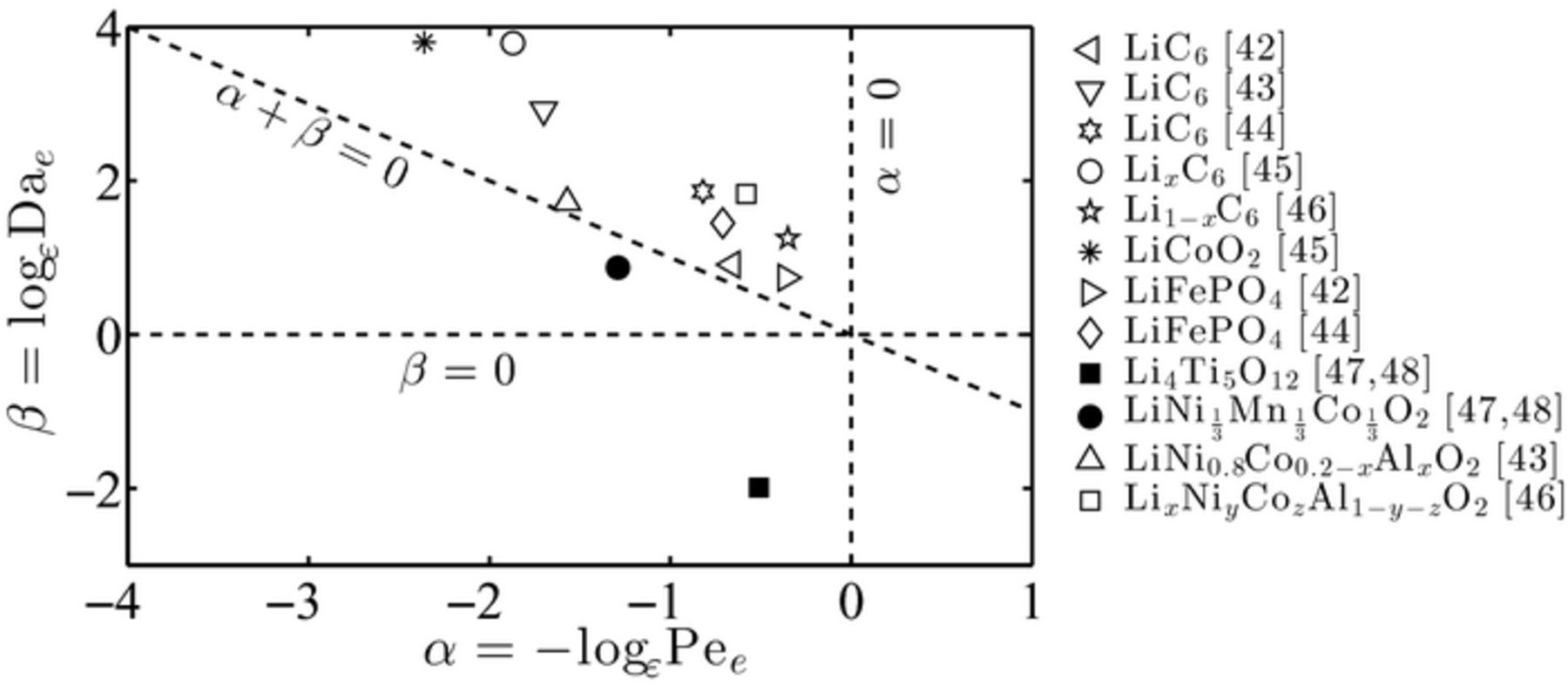
Figure 3. Values of the dimensionless parameters < ?CDAA$(α, β) for the most commonly used lithium-ion battery materials. These values, determined at room temperature (298 K), lie either inside the electrolyte applicability regime region (empty symbols) or outside (filled symbols).
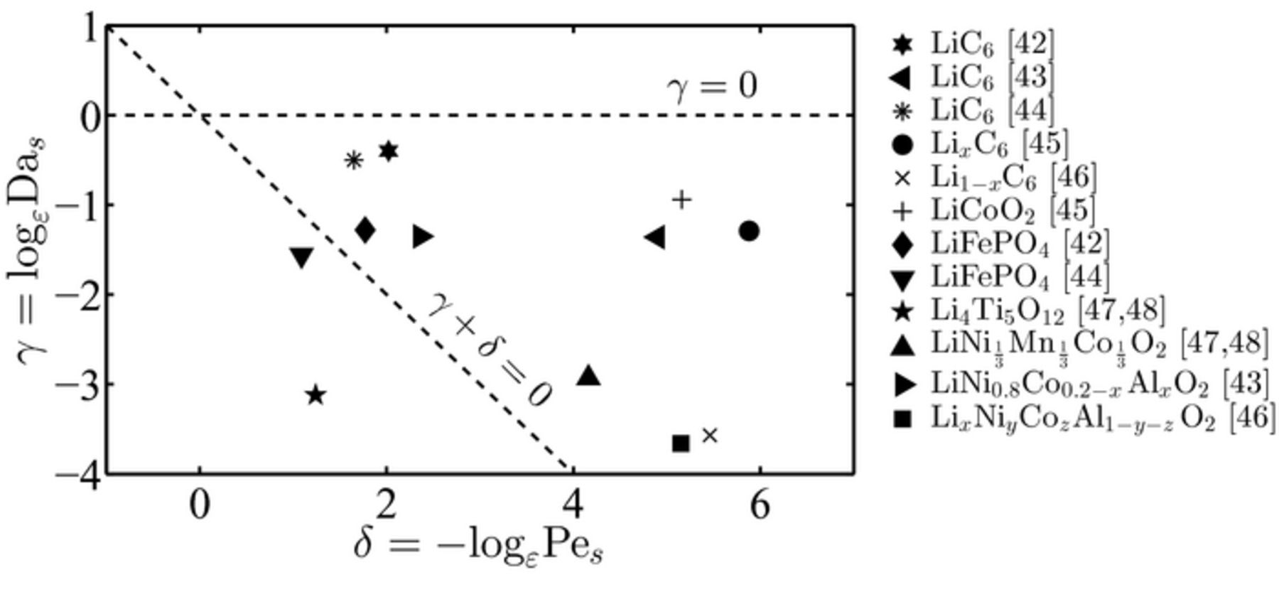
Figure 4. Values of the dimensionless parameters (δ, γ) for the most commonly used lithium-ion battery materials. These values, determined at room temperature (298 K), all lie outside the electrode applicability regime region.
Among the twelve chemistry considered in this analysis,45–51 ten possess electrolyte effective transport coefficients, i.e. dimensionless numbers (α, β), which do not violate the applicability conditions of macroscale models, see Figure 3. The theory developed previously ensures that the homogenized equations in the electrolyte will be able to accurately capture the dynamics at the pore-scale: this is consistent with the numerical simulations performed in Refs. 45–51, where Newman-type models have been successfully used to model transport in the electrolyte phase. On the contrary, two data points (solid symbols in Figure 3), corresponding to Li4Ti5O12 and LiNi1/3Mn1/3Co1/3O2 chemistry,50,51 lie outside the range of applicability. For these two chemistry, it is not guaranteed that the homogenized Equations (20) and (21) describing transport in the electrolyte will be effective in capturing pore-scale transport processes. Again, this is confirmed by the results presented in Refs. 50, 51, where a Newman-type model response could not properly capture experimental data, see Fig. 6 in Ref. 51. Such a discrepancy is understandable: Li4Ti5O12 has a very fast intercalation reaction rate (between 6 and 9 orders of magnitude faster than the other chemistry) which leads to mass transport limitations (or reaction-dominated regimes) and lack of pore-scale mixing.
Figure 4 shows the data points corresponding to the (δ, γ) values for the battery chemistry electrodes listed in Table I and calculated in Table II. All the data points lie outside the range of applicability of the upscaled equations of lithium-ion transport in the electrode phase, therefore suggesting that full pore-scale models have to be employed to accurately capture lithium-ion transport in the active particles. This is consistent with the numerical approaches used in Refs. 45–51, where no upscaled model is used in the active particles and the transport in the solid electrode is solved at the microscale. It is worth noticing that, since bounds on α, β, γ and δ have to be concurrently satisfied, the numerical simulations matched well the experiments only when the conditions on (α, β) were not violated, as discussed previously.
Operating conditions' dependence of macroscale models
Figures 3 and 4 showed the distribution of the dimensionless transport parameters α, β, γ and δ at room temperature in the phase diagrams and allowed one to a priori assess the validity of Newman-type models across different battery chemistry. These models, on the other hand, might also fail when used for the proper chemistry (i.e., the chemistry for which the corresponding α and β data points fall in the applicability regime regions at room temperature) but improper operating conditions. For this reason, the veracity of the upscaled equations of mass and charge transport in the electrolyte across battery cell operating conditions is also investigated. In particular, the study conducted in this section focuses on temperature and C-rate of operation and uses the electrode-electrolyte system described in Ref. 52. In this work, the authors compared the performance of their (continuum-scale) numerical simulations with experimental data for lithium-ion cells with LiyMn2O4 and LiNi0.8Co0.15Al0.05O2 cathode materials tested at different C-rate ranging from C/25 to 10C. We conduct our analysis for the case of LiyMn2O4 cathode material, but similar results can be easily extended to the LiNi0.8Co0.15Al0.05O2 case.
The case study analysis relies on the premise that temperature is one of the primary factors that influences the ability of the macroscale transport equations to capture battery dynamics at high C-rate. In fact, the battery cell temperature influences the transport parameters in the electrolyte phase. Those parameters are: k (reaction rate constant), De (the electrolyte diffusion coefficient), and Ke (the electrolyte conductivity coefficient). When the influence of temperature on k is much more pronounced than on De and Ke, as we will verify in the case of a battery operating at high C-rate, diffusion is no longer the dominant mode of transport. In this case the homogenized transport equations do not accurately capture transport at the microscale.
A single and constant value for the reaction rate k was considered in Ref. 52. Yet, experimental evidence shows significant cell temperature variations in terms of C-rate.53–58 Our analysis is conducted for three different C-rate: low (C/25), medium (1C), and high (10C). Following experimental data,53–58 the temperature increase, starting from room tenperature, can be estimated as follows: from 298 K to 299 K, from 298 K to 306 K, and from 298 K to 333 K at a discharge C-rate of C/25, 1C and 10C, respectively. We estimate the reaction rate constant kref at room temperature Tref = 298 K through
![Equation ([30])](https://content.cld.iop.org/journals/1945-7111/162/10/A1940/revision1/jes_162_10_A1940eqn41.jpg)
where Iapp (A/m2), the applied current density, is provided in Ref. 59 for each C-rate, see Table III. The electrochemical reaction rate constant k(T) for a given electrode system can be described as a function of temperature using the Arrhenius equation, as reported in Ref. 60:
![Equation ([31])](https://content.cld.iop.org/journals/1945-7111/162/10/A1940/revision1/jes_162_10_A1940eqn42.jpg)
where k(T) is the reaction rate constant of a given electrode at the desired temperature T. In (31), Ear is the electrode reaction rate activation energy. We set Ear = 78.24 kJ/mol at a reference temperature of 298 K.61 Using (31), we compute the values of k for different temperature conditions, which are then used to determine the parameter values α and β.
Table III. Reference reaction rate constants kref for lithium manganate cathode in terms of applied current Iapp.
| C-rate [1/h] | Iapp [A/m2] | kref [A · m · mol− 1] |
|---|---|---|
| C/25 | 0.34 | 2.03e-5 |
| 1C | 8.5 | 5.07e-4 |
| 10C | 85 | 5.07e-3 |
Similarly, the diffusion and conductivity coefficients, De and Ke, vary as a function of both temperature and the lithium concentration in the electrolyte phase. For the estimate of De and Ke at the reference temperature Tref, we use the same approach used in Ref. 52, where:
![Equation ([32])](https://content.cld.iop.org/journals/1945-7111/162/10/A1940/revision1/jes_162_10_A1940eqn43.jpg)
![Equation ([33])](https://content.cld.iop.org/journals/1945-7111/162/10/A1940/revision1/jes_162_10_A1940eqn44.jpg)
where we set  mol/m3 (d). This leads to reference values of 2.41e-10 m2/s and 0.922 S/m for De and Ke, respectively. Since, to the best of our knowledge, no analytical dependence on temperature is available for De and Ke, we use instead a curve fitting procedure from Figures 13 and 14 in Ref. 62 to determine De(T) and Ke(T). A summary of the estimated parameters for different C-rate and temperature ranges is given in Table IV.
Table IV. Dimensionless transport parameters of LiyMn2O4 cathode for different C-rate and temperatures.
| C-rate [1/h] | ℓ [m] | L [m] | ε [-] | k [A · m · mol− 1] | T [K] | De [m2sec− 1] | Ke [Ω− 1m− 1] | Dae [-] | Pee [-] | α [-] | β [-] |
|---|---|---|---|---|---|---|---|---|---|---|---|
| C/25 | 3.4e-6 | 1e-4 | 0.034 | 2.03e-5 | 298 | 2.41e-10 | 0.922 | 8.72e-5 | 4.26e-2 | −0.93 | 2.76 |
| C/25 | 3.4e-6 | 1e-4 | 0.034 | 2.07e-5 | 298.2 | 2.41e-10 | 0.922 | 8.91e-5 | 4.26e-2 | −0.93 | 2.76 |
| C/25 | 3.4e-6 | 1e-4 | 0.034 | 2.12e-5 | 298.4 | 2.41e-10 | 0.922 | 9.1e-5 | 4.27e-2 | −0.93 | 2.75 |
| C/25 | 3.4e-6 | 1e-4 | 0.034 | 2.16e-5 | 298.6 | 2.41e-10 | 0.922 | 9.29e-5 | 4.27e-2 | −0.93 | 2.75 |
| C/25 | 3.4e-6 | 1e-4 | 0.034 | 2.25e-5 | 299.0 | 2.41e-10 | 0.922 | 9.69e-5 | 4.27e-2 | −0.93 | 2.73 |
| 1C | 3.4e-6 | 1e-4 | 0.034 | 5.07e-4 | 298 | 2.41e-10 | 0.922 | 2.18e-3 | 4.26e-2 | −0.93 | 1.81 |
| 1C | 3.4e-6 | 1e-4 | 0.034 | 6.26e-4 | 300 | 2.55e-10 | 0.972 | 2.55e-3 | 4.28e-2 | −0.93 | 1.77 |
| 1C | 3.4e-6 | 1e-4 | 0.034 | 7.70e-4 | 302 | 2.69e-10 | 1.022 | 2.97e-3 | 4.29e-2 | −0.93 | 1.72 |
| 1C | 3.4e-6 | 1e-4 | 0.034 | 9.45e-4 | 304 | 2.82e-10 | 1.072 | 3.47e-3 | 4.31e-2 | −0.93 | 1.67 |
| 1C | 3.4e-6 | 1e-4 | 0.034 | 1.16e-3 | 306 | 2.96e-10 | 1.122 | 4.05e-3 | 4.33e-2 | −0.93 | 1.63 |
| 10C | 3.4e-6 | 1e-4 | 0.034 | 5.07e-3 | 298 | 2.41e-10 | 0.922 | 2.18e-2 | 4.26e-2 | −0.93 | 1.13 |
| 10C | 3.4e-6 | 1e-4 | 0.034 | 8.54e-3 | 303 | 2.75e-10 | 1.047 | 3.21e-2 | 4.30e-2 | −0.93 | 1.02 |
| 10C | 3.4e-6 | 1e-4 | 0.034 | 2.30e-2 | 313 | 3.44e-10 | 1.297 | 6.93e-2 | 4.41e-2 | −0.92 | 0.79 |
| 10C | 3.4e-6 | 1e-4 | 0.034 | 5.84e-2 | 323 | 4.13e-10 | 1.547 | 1.47e-1 | 4.52e-2 | −0.92 | 0.57 |
| 10C | 3.4e-6 | 1e-4 | 0.034 | 1.40e-1 | 333 | 4.82e-10 | 1.797 | 3.01e-1 | 4.64e-2 | −0.91 | 0.35 |
Based on above calculations, we determine the temperature-dependent trajectories of the data points (α,β) computed at the temperature intervals characteristic of each C-rate. Table IV summarizes the variation of parameters α and β as a function of the operating conditions for the three C-rate of interest. The data points and their variation with temperature and C-rate are schematically represented in Figure 5.
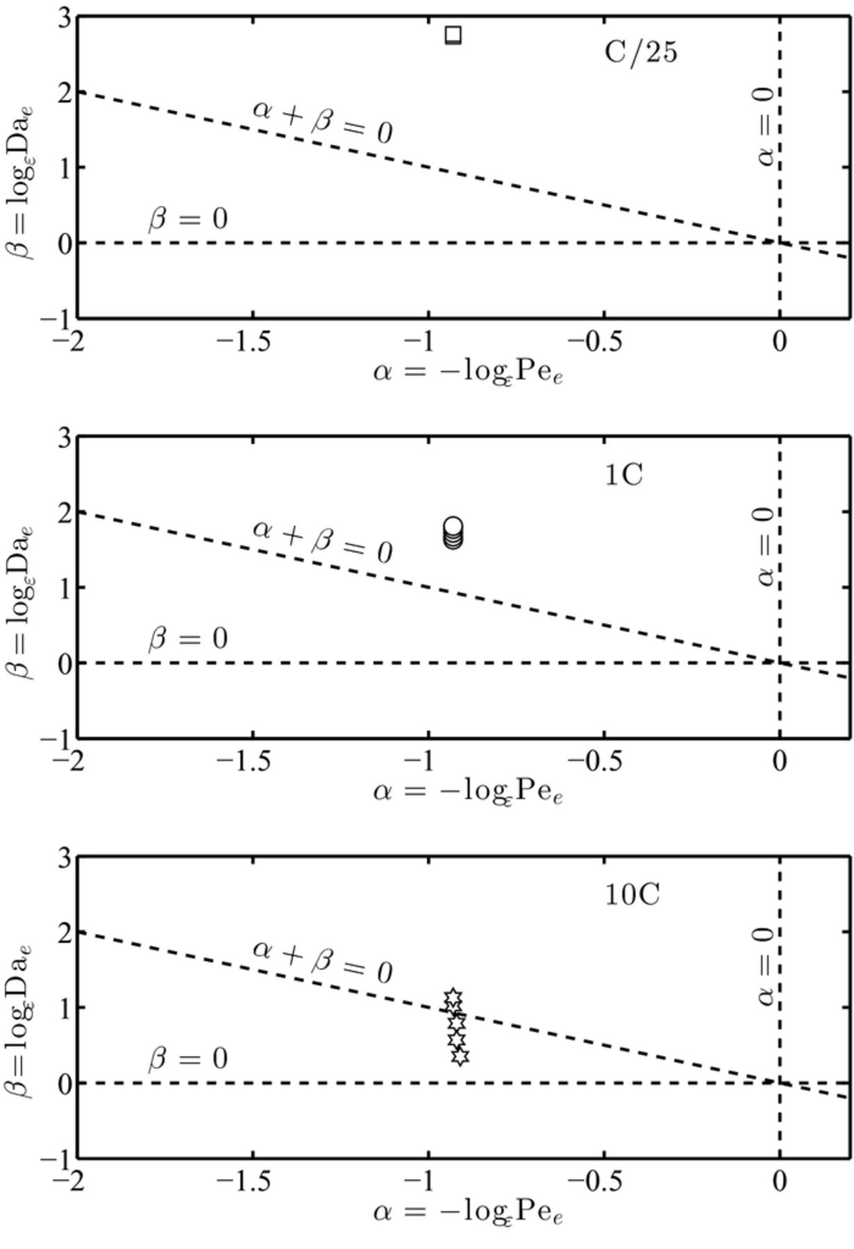
Figure 5. Variation with temperature of dimensionless parameters α and β in lithium manganate cathode batteries for three different C-rate of discharge, C/25 (top), 1C (middle) and 10C (bottom). An increase in C-rate induces higher operating temperature variations inside a battery: as a result the system can be driven outside the applicability regime region.
Figure 5 (top) shows that at a C/25 rate of discharge, there is minimal temperature increase over the duration of a discharge event. The magnitude of parameter α remains invariant, while β increases slightly due to an increase in the Dae number. The behavior of the system (as a function of temperature) is linear with β. The data points satisfy the constraints on α and β. Hence, the upscaled equations for lithium mass transport should provide an accurate description of the pore scale behavior. This is consistent with the simulation results from a continuum-scale simulator obtained in Figure 7(a) of Ref. 52, where there is a perfect match between the model and the experimental response.
At a 1C rate of discharge, Figure 4 (middle), there is a moderate increase in temperature over the duration of the simulation cycle. The magnitude of parameter α remains invariant, while β increases at a moderate rate due to a faster increase in the Dae number. The behavior of this system is linear in α and β. At elevated temperatures, the effect of increase in the reaction rate constant k dominates any increase of De and Ke. The data points satisfy the constraints on α and β over the range of operating temperature conditions. Hence the homogenized set of transport equations used in Ref. 52, Figure 7(a), still provides an accurate description of the pore scale behavior, leading to good correlation with experimental data.
At a 10C rate of discharge, there is a very significant increase in the battery temperature over the operating conditions. There is a very small increase in α as the increase in De marginally dominates the increase in Ke, leading to an incremental increase in the Pee number. The reaction rate constant is 2 to 3 orders of magnitude higher than at lower C-rate; hence, the rate of decrease in β is higher than the rate of increase in α. For the LiMn2O4 cathode system, the macroscale transport equations are no longer accurate in describing microscale transport processes at temperatures 313 K or higher. This is because the value of α + β is less than 0, which violates one of the three constraints on these two parameters. At high operating temperatures and C-rate, the lithium manganate cathode system operates in a transport regime where the three lithium transport processes (reaction, diffusion, and electro-migration) are of the same order. In this scenario, very fast reaction kinetics lead to diffusion-limited regimes where diffusion is no longer the dominant transport mechanism in the medium. As a result, macroscale equations describing electrolyte transport are vulnerable and can be invalidated due to lack of scale separation with respect to the pore-scale.
The performance prediction of continuum-scale models based on the phase diagram Figure 4 (bottom) is, again, consistent with the analysis performed in Ref. 52, Figure 7(a), where the numerical solution obtained from macroscopic models cannot capture the experimental results. Under these circumstances, a multi-scale model is necessary to incorporate the effects of transport both at the pore-scale and the macroscopic scale.
The approach implemented above is significant in terms of identifying the temperature of operation and C-rate of current charge/discharge as crucial parameters dictating the dominance of one transport mechanism over the other(s) in the battery electrode/electrolyte medium. Standard Newman-type macroscopic models under scenarios similar to the one described above are invalid and may fail to capture microscale transport processes.
Conclusions
Lithium-ion transport in batteries involves diffusion, electromigration and heterogeneous intercalation reactions occurring in geometrically complex porous electrodes. As such, ion transport can be modeled on a multiplicity of scales, ranging from the pore- to the system-scale. Macroscopic models, which are approximate representations of the pore-scale physics, are advantageous due to their simplicity (relative to fully pore-scale descriptions) and their limited computational burden. These two aspects render them particularly appealing for PDE-based control and estimation strategies of SOH and SOC. Yet, macroscale models are known to fail as predictive tools under given operating conditions, e.g. high C-rate and high temperature. This hampers any control and design strategies based on them.
In this work we establish the robustness of macroscopic diffusion-migration-reaction (DRM) equations that describe the evolution of mean (spatially averaged) lithium-ion concentration and potential in the electrolyte and electrode phases, treated as overlapping continua. Starting from the equations describing lithium-ion transport at the pore-scale, we use multiple scale expansions to rigorously derive macroscopic dual-continua models and identify under which conditions they describe micro-scale dynamics with the accuracy prescribed by the homogenization technique. The relative importance between diffusion, conduction, and reaction can be quantified by electric Péclet Pej and Damköhler Daj, j = {e, s}, numbers in the electrolyte and electrode phases.
Our main result, summarized in the two (Da,Pe)-phase diagrams, is the identification of the sufficient conditions needed to guarantee that the pore- and the continuum-scales can be separated and the system of macroscopic diffusion-reaction-migration Equations (20)-(21) and (26)-(27) accurately represents pore scale processes. Such conditions are expressed in terms of bounds on the order of magnitude of Pej and Daj, j = {e, s} and indicate that there may be entire classes of battery chemistry for which macroscopic models are not accurate descriptors of micro-scale dynamics.
We showed the distribution of parameters Pej and Daj in the electrolyte and electrode phase diagrams for different chemical compositions of the most common commercial batteries, for which the transport parameters have been experimentally determined or estimated based on analytical techniques for the purpose of numerical simulations. More importantly, we validated the new conditions over a case study, where we have determined the transport parameters Pee and Dae (or α and β) in the electrolyte phase diagram for different operating conditions based on battery chemistry composition, temperature and C-rate. The performance predictions of continuum models based on a phase diagram analysis confirmed the results independenently obtained from other numerical and experimental studies, i.e. a breakdown of continuum models at high C-rate.
Bounds on parameters Pej and Daj, j = {e, s} also highlight the importance of mixing at the sub-pore scale for continuum equations to be valid. In this regard, diffusion-limited regimes due to either fast reaction kinetics (e.g. at high operating temperatures) and/or fast electromigration are the critical scenarios where separation of scales may lack and continuum models be invalidated. Models that account for a full coupling between the two scales must be employed instead,63 and replace classical continuum models (e.g. single particle models) if accurate predictions of the battery response under different operating conditions are sought.
To the best of our knowledge, the literature lacks in such a systematic method to guide researchers in the use of the correct modeling tools for battery systems. Future SOH and SOC estimations based on macroscopic models should account for model robustness and error, whenever scale separation cannot be guaranteed, e.g., at high C-rate.
: Appendix A: Homogenization in the Electrolyte
We set cjε(x, t) = cj(x, y, t, τr, τme, τms) and ϕjε(x, t) = ϕj(x, y, t, τr, τme, τms), j = {e, s}. Then, combining (17) with (8a) and (8b) we obtain
![Equation ([A1])](https://content.cld.iop.org/journals/1945-7111/162/10/A1940/revision1/jes_162_10_A1940eqn45.jpg)
and
![Equation ([A2])](https://content.cld.iop.org/journals/1945-7111/162/10/A1940/revision1/jes_162_10_A1940eqn46.jpg)
for  , subject to
![Equation ([A3])](https://content.cld.iop.org/journals/1945-7111/162/10/A1940/revision1/jes_162_10_A1940eqn47.jpg)
and
![Equation ([A4])](https://content.cld.iop.org/journals/1945-7111/162/10/A1940/revision1/jes_162_10_A1940eqn48.jpg)
respectively, where f(ceε, csε, ϕsε, ϕeε) is defined in (10).
Appendix. Mass and charge transport asymptotic expansions
Substituting (18) and (19) into the mass transport equation in the electrolyte (8) leads to
![Equation ([A5])](https://content.cld.iop.org/journals/1945-7111/162/10/A1940/revision1/jes_162_10_A1940eqn49.jpg)
where the nonlinear term in (8) is expanded in a Mclaurin series
![Equation ([A6])](https://content.cld.iop.org/journals/1945-7111/162/10/A1940/revision1/jes_162_10_A1940eqn50.jpg)
Similarly, the interface condition (A3) can be written as
![Equation ([A7])](https://content.cld.iop.org/journals/1945-7111/162/10/A1940/revision1/jes_162_10_A1940eqn51.jpg)
since  , where
![Equation ([A8a])](https://content.cld.iop.org/journals/1945-7111/162/10/A1940/revision1/jes_162_10_A1940eqn52.jpg)
![Equation ([A8b])](https://content.cld.iop.org/journals/1945-7111/162/10/A1940/revision1/jes_162_10_A1940eqn53.jpg)
![Equation ([A8c])](https://content.cld.iop.org/journals/1945-7111/162/10/A1940/revision1/jes_162_10_A1940eqn54.jpg)
![Equation ([A8d])](https://content.cld.iop.org/journals/1945-7111/162/10/A1940/revision1/jes_162_10_A1940eqn55.jpg)
Combining (18) and (19) with the charge transport Equation (A2) and boundary condition (A4) yields to
![Equation ([A9])](https://content.cld.iop.org/journals/1945-7111/162/10/A1940/revision1/jes_162_10_A1940eqn56.jpg)
subject to
![Equation ([A10])](https://content.cld.iop.org/journals/1945-7111/162/10/A1940/revision1/jes_162_10_A1940eqn57.jpg)
where A0, A1, B0 and B1 are defined in (A8). Next, we compare terms of like-order of ε.
Appendix. Terms of order

Collecting the leading-order terms in the mass transport equation and corresponding boundary condition (A5) and (A7) respectively, we obtain
![Equation ([A11])](https://content.cld.iop.org/journals/1945-7111/162/10/A1940/revision1/jes_162_10_A1940eqn58.jpg)
subject to
![Equation ([A12])](https://content.cld.iop.org/journals/1945-7111/162/10/A1940/revision1/jes_162_10_A1940eqn59.jpg)
Similarly, at the leading order the charge transport equation is
![Equation ([A13])](https://content.cld.iop.org/journals/1945-7111/162/10/A1940/revision1/jes_162_10_A1940eqn60.jpg)
subject to
![Equation ([A14])](https://content.cld.iop.org/journals/1945-7111/162/10/A1940/revision1/jes_162_10_A1940eqn61.jpg)
Homogeneity of (A11)-(A12) and (A13)-(A14), guarantees that ce0 and ϕe0 are independent of y, i.e.
![Equation ([A15])](https://content.cld.iop.org/journals/1945-7111/162/10/A1940/revision1/jes_162_10_A1940eqn62.jpg)
![Equation ([A16])](https://content.cld.iop.org/journals/1945-7111/162/10/A1940/revision1/jes_162_10_A1940eqn63.jpg)
Appendix. Terms of order

Since ∇yce0 ≡ 0 and ∇yϕe0 ≡ 0, the mass balance equation (A5) at order  simplifies to
![Equation ([A17])](https://content.cld.iop.org/journals/1945-7111/162/10/A1940/revision1/jes_162_10_A1940eqn64.jpg)
subject to the interface condition
![Equation ([A18])](https://content.cld.iop.org/journals/1945-7111/162/10/A1940/revision1/jes_162_10_A1940eqn65.jpg)
Integrating (A17) over  with respect to y, while accounting for the boundary condition (A18), and the periodicity of the coefficients on the external boundary of the unit cell ∂Y, we obtain
![Equation ([A19])](https://content.cld.iop.org/journals/1945-7111/162/10/A1940/revision1/jes_162_10_A1940eqn66.jpg)
where  is defined by (23).
Combining (A19) with (A17) to eliminate the temporal derivative, we obtain
![Equation ([A20])](https://content.cld.iop.org/journals/1945-7111/162/10/A1940/revision1/jes_162_10_A1940eqn67.jpg)
Similarly, the charge balance equation (A9) at  is
is
![Equation ([A21])](https://content.cld.iop.org/journals/1945-7111/162/10/A1940/revision1/jes_162_10_A1940eqn68.jpg)
subject to
![Equation ([A22])](https://content.cld.iop.org/journals/1945-7111/162/10/A1940/revision1/jes_162_10_A1940eqn69.jpg)
for y ∈ Γ. Equations (A18), (A20), (A21) and (A22) form boundary value problems for both ce1 and ϕe1. Following Ref. 64 and Ref. 27 (pp. 10, Eqs. 3.6–3.7), we look for solutions in the form
![Equation ([A23])](https://content.cld.iop.org/journals/1945-7111/162/10/A1940/revision1/jes_162_10_A1940eqn70.jpg)
Substitution of (A23) into (A20) and (A18) leads to
![Equation ([A24a])](https://content.cld.iop.org/journals/1945-7111/162/10/A1940/revision1/jes_162_10_A1940eqn71.jpg)
subject to  and
and
![Equation ([A24b])](https://content.cld.iop.org/journals/1945-7111/162/10/A1940/revision1/jes_162_10_A1940eqn72.jpg)
where I is the identity matrix, and  and
and  are periodic vector fields. Substitution of (A23) into (A21) and (A22) leads to
![Equation ([A25a])](https://content.cld.iop.org/journals/1945-7111/162/10/A1940/revision1/jes_162_10_A1940eqn73.jpg)
subject to
![Equation ([A25b])](https://content.cld.iop.org/journals/1945-7111/162/10/A1940/revision1/jes_162_10_A1940eqn74.jpg)
Equations (A24) and (A25) define the closure variables  and
and  . The coupling of
  and
and  with ce0(x), ϕe0(x), A0(x) and B0(x) through the boundary value problems (A24) and (A25) is incompatible with the closure variables' general representation postulated in (A23). This inconsistency is resolved by imposing the following constraints on the exponents α and β. If we choose β > max {0, −α} and α < 0, then the term
  is negligible relative to the smallest term in (A24) and the nonlinear migration term ε− αλt2+Ke/c0e relative to De. Under these constraints, (A24) and (A25) simplify to
![Equation ([A26a])](https://content.cld.iop.org/journals/1945-7111/162/10/A1940/revision1/jes_162_10_A1940eqn75.jpg)
![Equation ([A26b])](https://content.cld.iop.org/journals/1945-7111/162/10/A1940/revision1/jes_162_10_A1940eqn76.jpg)
Equation (A26) can be satisfied for all x ∈ Ω if
![Equation ([A27a])](https://content.cld.iop.org/journals/1945-7111/162/10/A1940/revision1/jes_162_10_A1940eqn77.jpg)
![Equation ([A27b])](https://content.cld.iop.org/journals/1945-7111/162/10/A1940/revision1/jes_162_10_A1940eqn78.jpg)
Similarly, (A25) yields
![Equation ([A28a])](https://content.cld.iop.org/journals/1945-7111/162/10/A1940/revision1/jes_162_10_A1940eqn79.jpg)
![Equation ([A28b])](https://content.cld.iop.org/journals/1945-7111/162/10/A1940/revision1/jes_162_10_A1940eqn80.jpg)
and
![Equation ([A29a])](https://content.cld.iop.org/journals/1945-7111/162/10/A1940/revision1/jes_162_10_A1940eqn81.jpg)
![Equation ([A29b])](https://content.cld.iop.org/journals/1945-7111/162/10/A1940/revision1/jes_162_10_A1940eqn82.jpg)
Consistency of (A27) with (A28) implies
![Equation ([A30a])](https://content.cld.iop.org/journals/1945-7111/162/10/A1940/revision1/jes_162_10_A1940eqn83.jpg)
![Equation ([A30b])](https://content.cld.iop.org/journals/1945-7111/162/10/A1940/revision1/jes_162_10_A1940eqn84.jpg)
In (A29), the conductivity tensor Ke is a function of concentration ce and potential ϕe. With an order ε approximation Ke ≈ Ke(ce0, ϕe0). Then, (A29) can be simplified to
![Equation ([A31a])](https://content.cld.iop.org/journals/1945-7111/162/10/A1940/revision1/jes_162_10_A1940eqn85.jpg)
![Equation ([A31b])](https://content.cld.iop.org/journals/1945-7111/162/10/A1940/revision1/jes_162_10_A1940eqn86.jpg)
As a result,  . The treatment of the closure variable is consistent with the approach employed in Ref. 65. The closure variable
  defines the cell problem and describes the behavior of the effective diffusion and conductivity tensors.
Recalling the definitions of Dae and Pee in (19) allows us to reformulate the conditions in terms of α and β in the form of constraints 2)–4) for the electrolyte. Having identified the conditions that guarantee homogenizability, we proceed to derive the effective mass transport equation (20).
Appendix. Terms of order

Collecting the zeroth-order term in the mass balance equation (A5) and first-order term in the corresponding boundary condition (A7), we obtain
![Equation ([A32])](https://content.cld.iop.org/journals/1945-7111/162/10/A1940/revision1/jes_162_10_A1940eqn87.jpg)
subject to
![Equation ([A33])](https://content.cld.iop.org/journals/1945-7111/162/10/A1940/revision1/jes_162_10_A1940eqn88.jpg)
since ∇yce0 = 0. Integrating (A32) over  with respect to y and using the boundary condition (A33) leads to
![Equation ([A34])](https://content.cld.iop.org/journals/1945-7111/162/10/A1940/revision1/jes_162_10_A1940eqn89.jpg)
where  ,
,  ,
,  and
and
![Equation ([A35a])](https://content.cld.iop.org/journals/1945-7111/162/10/A1940/revision1/jes_162_10_A1940eqn90.jpg)
![Equation ([A35b])](https://content.cld.iop.org/journals/1945-7111/162/10/A1940/revision1/jes_162_10_A1940eqn91.jpg)
Next, we recall that
![Equation ([A36])](https://content.cld.iop.org/journals/1945-7111/162/10/A1940/revision1/jes_162_10_A1940eqn92.jpg)
Multiplying the temporal derivative of (A36) by ε, we obtain
![Equation ([A37])](https://content.cld.iop.org/journals/1945-7111/162/10/A1940/revision1/jes_162_10_A1940eqn93.jpg)
Multiplying (A34) by ε, adding the result to (A19), and using (A37), we obtain
![Equation ([A38])](https://content.cld.iop.org/journals/1945-7111/162/10/A1940/revision1/jes_162_10_A1940eqn94.jpg)
Combining this result with the expansions  and
and  while recalling the definitions of Dae and Pee in (19) and assuming
  and
and  , where ψ = {c, ϕ}, leads to
![Equation ([A39])](https://content.cld.iop.org/journals/1945-7111/162/10/A1940/revision1/jes_162_10_A1940eqn95.jpg)
since
![Equation ([A40])](https://content.cld.iop.org/journals/1945-7111/162/10/A1940/revision1/jes_162_10_A1940eqn96.jpg)
where  is defined by (22).
Similarly, collecting  terms in the charge balance equation in the electrolyte (A9) and
  terms in the boundary condition (A10) while accounting for ∇yce0 = 0, we obtain
![Equation ([A41])](https://content.cld.iop.org/journals/1945-7111/162/10/A1940/revision1/jes_162_10_A1940eqn97.jpg)
subject to
![Equation ([A42])](https://content.cld.iop.org/journals/1945-7111/162/10/A1940/revision1/jes_162_10_A1940eqn98.jpg)
We multiply by ε both Equation (A41) and its boundary condition (A42), add them to (A21) and (A22), respectively, and integrate the resulting equation over  while employing the newly obtained boundary conditions. This leads to
![Equation ([A43])](https://content.cld.iop.org/journals/1945-7111/162/10/A1940/revision1/jes_162_10_A1940eqn99.jpg)
where  . Following a similar procedure to that outlined for the mass transport equation, (A43) can be written as
![Equation ([A44])](https://content.cld.iop.org/journals/1945-7111/162/10/A1940/revision1/jes_162_10_A1940eqn100.jpg)
where  is defined by (22).
Equations (A39) and (A44) govern the dynamics of  and
and  in the electrolyte up to errors of order ε2.
: Appendix B: Homogenization in the Electrode
We follow the same procedure as outlined in Appendix A. We report the derivations for completeness. We set cjε(x, t) = cj(x, y, t, τr, τme, τms) and ϕjε(x, t) = ϕj(x, y, t, τr, τme, τms), j = {e, s}. Then, combining (17) with (11) and (12) we obtain
![Equation ([B1])](https://content.cld.iop.org/journals/1945-7111/162/10/A1940/revision1/jes_162_10_A1940eqn101.jpg)
and
![Equation ([B2])](https://content.cld.iop.org/journals/1945-7111/162/10/A1940/revision1/jes_162_10_A1940eqn102.jpg)
subject to
![Equation ([B3])](https://content.cld.iop.org/journals/1945-7111/162/10/A1940/revision1/jes_162_10_A1940eqn103.jpg)
and
![Equation ([B4])](https://content.cld.iop.org/journals/1945-7111/162/10/A1940/revision1/jes_162_10_A1940eqn104.jpg)
respectively, where f(ceε, csε, ϕsε, ϕeε) is defined in (10).
Appendix. Mass and charge transport asymptotic expansions
Substituting (18) and (19) into the mass transport equation in the electrode (B1), we obtain
![Equation ([B5])](https://content.cld.iop.org/journals/1945-7111/162/10/A1940/revision1/jes_162_10_A1940eqn105.jpg)
subject to
![Equation ([B6])](https://content.cld.iop.org/journals/1945-7111/162/10/A1940/revision1/jes_162_10_A1940eqn106.jpg)
where A0, A1, B0 and B1 are defined in (A8). Similarly, the charge transport equation (B2) and the boundary condition (B4) combined with (18) and (19) yield to
![Equation ([B7])](https://content.cld.iop.org/journals/1945-7111/162/10/A1940/revision1/jes_162_10_A1940eqn107.jpg)
subject to
![Equation ([B8])](https://content.cld.iop.org/journals/1945-7111/162/10/A1940/revision1/jes_162_10_A1940eqn108.jpg)
Appendix. Terms of order

Collecting the leading-order terms in the mass transport equation and corresponding boundary conditions (B5) and (B6), we obtain
![Equation ([B9])](https://content.cld.iop.org/journals/1945-7111/162/10/A1940/revision1/jes_162_10_A1940eqn109.jpg)
subject to the interface condition
![Equation ([B10])](https://content.cld.iop.org/journals/1945-7111/162/10/A1940/revision1/jes_162_10_A1940eqn110.jpg)
Similarly, at the leading order the charge balance equation (B7) and the boundary condition yield
![Equation ([B11])](https://content.cld.iop.org/journals/1945-7111/162/10/A1940/revision1/jes_162_10_A1940eqn111.jpg)
subject to
![Equation ([B12])](https://content.cld.iop.org/journals/1945-7111/162/10/A1940/revision1/jes_162_10_A1940eqn112.jpg)
The homogeneity of Equations (B9)–(B12) ensures that the above boundary value problems have both a trivial solution, i.e.
![Equation ([B13a])](https://content.cld.iop.org/journals/1945-7111/162/10/A1940/revision1/jes_162_10_A1940eqn113.jpg)
![Equation ([B13b])](https://content.cld.iop.org/journals/1945-7111/162/10/A1940/revision1/jes_162_10_A1940eqn114.jpg)
Appendix. Terms of order

At the following order, the mass transport equation (B5) can be written as
![Equation ([B14])](https://content.cld.iop.org/journals/1945-7111/162/10/A1940/revision1/jes_162_10_A1940eqn115.jpg)
since ∇ycs0 ≡ 0, and it is subject to the boundary condition
![Equation ([B15])](https://content.cld.iop.org/journals/1945-7111/162/10/A1940/revision1/jes_162_10_A1940eqn116.jpg)
Integrating (B14) over  with respect to y, while accounting for the boundary condition (B15), and the periodicity of the coefficients on the external boundary of the unit cell ∂Y, we obtain
![Equation ([B16])](https://content.cld.iop.org/journals/1945-7111/162/10/A1940/revision1/jes_162_10_A1940eqn117.jpg)
We combine (B16) with (B14) to eliminate the temporal derivative and obtain
![Equation ([B17])](https://content.cld.iop.org/journals/1945-7111/162/10/A1940/revision1/jes_162_10_A1940eqn118.jpg)
Similarly, the order  of the charge balance equation (B7) can be simplified to
![Equation ([B18])](https://content.cld.iop.org/journals/1945-7111/162/10/A1940/revision1/jes_162_10_A1940eqn119.jpg)
subject to
![Equation ([B19])](https://content.cld.iop.org/journals/1945-7111/162/10/A1940/revision1/jes_162_10_A1940eqn120.jpg)
Equations (B17) and (B18) subject to (B15) and (B19) form a boundary value problem for cs1 and ϕs1, respectively. As outlined in Appendix A, we look for a solution in the form
![Equation ([B20])](https://content.cld.iop.org/journals/1945-7111/162/10/A1940/revision1/jes_162_10_A1940eqn121.jpg)
Substitution of (B20) into (B17) and (B15) leads to the following cell problem for the closure variable  ,
,
![Equation ([B21a])](https://content.cld.iop.org/journals/1945-7111/162/10/A1940/revision1/jes_162_10_A1940eqn122.jpg)
subject to  and
and
![Equation ([B21b])](https://content.cld.iop.org/journals/1945-7111/162/10/A1940/revision1/jes_162_10_A1940eqn123.jpg)
The boundary-value problem (B21) couples the pore scale with the continuum scale, in the sense that the closure variable  —a solution of the pore-scale cell problem (B21) —is influenced by the continuum scale through its dependence on the macroscopic concentration cs0(x). This coupling is incompatible with the general representation (B20). This inconsistency is resolved by imposing the following constraint on the exponent γ, namely γ > 0. This condition ensures that
  is independent of cs0, and the cell problem (B21) can be simplified to
![Equation ([B22a])](https://content.cld.iop.org/journals/1945-7111/162/10/A1940/revision1/jes_162_10_A1940eqn124.jpg)
![Equation ([B22b])](https://content.cld.iop.org/journals/1945-7111/162/10/A1940/revision1/jes_162_10_A1940eqn125.jpg)
Similarly, substitution of (B20) into the  -charge balance equation (B18) and its boundary condition (B19) leads to the following cell problem for the closure variable
  ,
,
![Equation ([B23a])](https://content.cld.iop.org/journals/1945-7111/162/10/A1940/revision1/jes_162_10_A1940eqn126.jpg)
subject to  and
and
![Equation ([B23b])](https://content.cld.iop.org/journals/1945-7111/162/10/A1940/revision1/jes_162_10_A1940eqn127.jpg)
where  is a Y-periodic vector field. Separation between pore- and continuum-scales requires γ + δ > 0. Under this condition (B23), simplifies to
![Equation ([B24a])](https://content.cld.iop.org/journals/1945-7111/162/10/A1940/revision1/jes_162_10_A1940eqn128.jpg)
![Equation ([B24b])](https://content.cld.iop.org/journals/1945-7111/162/10/A1940/revision1/jes_162_10_A1940eqn129.jpg)
In (B22) and (B24), the diffusion and conductivity tensors are functions of concentration ce and potential ϕe. With an order ε approximation De ≈ De(ce0, ϕe0) and Ke ≈ Ke(ce0, ϕe0). Then,  , where
  is a solution of the closure problem
![Equation ([B25a])](https://content.cld.iop.org/journals/1945-7111/162/10/A1940/revision1/jes_162_10_A1940eqn130.jpg)
![Equation ([B25b])](https://content.cld.iop.org/journals/1945-7111/162/10/A1940/revision1/jes_162_10_A1940eqn131.jpg)
Appendix. Terms of order

At the leading order, the mass transport equation in the electrode (B5)
![Equation ([B26])](https://content.cld.iop.org/journals/1945-7111/162/10/A1940/revision1/jes_162_10_A1940eqn132.jpg)
subject to
![Equation ([B27])](https://content.cld.iop.org/journals/1945-7111/162/10/A1940/revision1/jes_162_10_A1940eqn133.jpg)
Integrating (B26) over  with respect to y and using the interface condition (B27) leads to
![Equation ([B28])](https://content.cld.iop.org/journals/1945-7111/162/10/A1940/revision1/jes_162_10_A1940eqn134.jpg)
where  . Similarly, the leading order of the charge transport equation is
![Equation ([B29])](https://content.cld.iop.org/journals/1945-7111/162/10/A1940/revision1/jes_162_10_A1940eqn135.jpg)
subject to
![Equation ([B30])](https://content.cld.iop.org/journals/1945-7111/162/10/A1940/revision1/jes_162_10_A1940eqn136.jpg)
Multiplying both (B29) and (B30) by ε, adding them to (B14) and (B15), respectively, and then integrating over  , we obtain
![Equation ([B31])](https://content.cld.iop.org/journals/1945-7111/162/10/A1940/revision1/jes_162_10_A1940eqn137.jpg)
where  .
.
Following the procedure outlined in Appendix A and assuming that  , Equations (B28) and (B31) lead to the macroscopic equations for mass and charge transport in the electrode (26) and (27), respectively.
Footnotes
- c
C-rate is defined as the rate of charge or discharge current in normalized form:
where I is the battery current and Qnom is the rated capacity of the battery. The general expression C/hh indicates that the number of hours to completely discharge the battery at a constant current is hh.38 - d
From Ref. 52,
varies in the range of 1,000 to 2,000 mol/m3 over the entire duration of the simulations.

